(click to view pdf)

Abstract:

\( \def\citeLevitt{{[2]}} \def\citeLevittThomas{{[3]}} \) When a defect potential is placed in a material, the material rearranges and the total potential at long-range is screened by the electrons. In the finite temperature reduced Hartree-Fock model, small defects are completely screened ; the total change in potential decays exponentially. On the other hand, in metals at zero temperature, the presence of the Fermi-surface introduces non-analytic behaviour into the independent-particle susceptibility $\chi_0$, leading to what are known as Friedel oscillations; the total potential oscillates and decays algebraically, with exponent depending on the dimensionality. \( \def\ep{{\varepsilon}} \def\bm{{\bf}} \def\si{{\mathrm{si}}} \def\coloneqq{:=} \)

Here, you can find links to the references that are cited in the poster:

References

1. Michael Greenblatt. Resolution of singularities, asymptotic expansions of integrals and related phenomena. Journal d’Analyse Mathematique 111.1 (2010), pp. 221–245. [doi][arXiv]
2. Antoine Levitt. Screening in the Finite-Temperature Reduced Hartree–Fock Model. Archive for Rational Mechanics and Analysis 238.2 (2020), pp. 901–927. [doi][arXiv]
3. Antoine Levitt and Jack Thomas. Locality in the reduced Hartree–Fock model. Unpublished manuscript.
4. Bogdan Mihaila. Lindhard function of a d-dimensional Fermi gas (2011). [link]
5. George E. Simion and Gabriele F. Giuliani. Friedel oscillations in a Fermi liquid. Physical Review B 72.4 (2005). [doi]
6. Elias M. Stein. Harmonic Analysis. Princeton University Press, Dec. 1993. [link]
7. Jens Lindhard. On the properties of a gas of charged particles. Dan. Mat. Fys. Medd. 28, no.8 (1954).
8. Table of Integrals, Series, and Products. Elsevier, 2015. [link]

---

Here are some additional details not on the poster, including a section on the results for the free elction gas:

Introduction

Suppose we have a lattice $\mathcal R \subset \mathbb R^d$ and an associated unit cell $\Gamma$. Define $L^2_{\mathrm{per}} \coloneqq \{ f \in L^2(\Gamma) \colon f \text{ is }\mathcal{R}\text{-periodic}\}$. For a fixed periodic potential $W_{\mathrm{per}} \in L^2_{\mathrm{per}}$, associated Fermi level $\ep_{\mathrm{F}}$, consider the response to an effective potential $V$: \begin{align} \rho_V(x) &= F_{\ep_{\mathrm{F}}}\big(-\Delta + W_{\mathrm{per}} +V \big)(x,x) \nonumber \\ % &= \rho_0(x) + \chi_0V(x) + \cdots \tag{1}\label{eq:rho-exp} \end{align} where $F_{\ep_{\mathrm{F}}}(x) \coloneqq \big( 1 + e^{\frac{x - \ep_{\mathrm{F}}}{k_\mathrm{B}T}}\big)^{-1}$ is the Fermi-Dirac distribution with temperature $T\geq0$ and $\chi_0$ is the independent particle susceptibility operator, describing the linear response to the density of a non-interacting system of electrons. In the linear model the interaction between the electrons is neglected and we consider $V = V_{\mathrm{def}}$, whereas the reduced Hartree-Fock model takes the form \begin{align} V = V_{\mathrm{def}} + \big( \rho_V - \rho_0 \big) \star |\,\cdot\,|^{-1}. \tag{2}\label{eq:rHF} \end{align}

Finite temperature

In the finite temperature case ($T>0$), the response $\rho_V - \rho_0$ decays "as quickly as" $V$: That is, we have \begin{gather} V \in L^2_N \,\,\Rightarrow\,\, \rho_V - \rho_0 \in L^2_N, \end{gather} where $L^2_N \coloneqq \{ \phi \colon (1 + |x|^2)^{\frac{N}{2}} \phi \in L^2\}$. Moreover, the asymptotic behaviour of $\rho_V - \rho_0$ is given by the first term of the expansion: \begin{align} \rho_V - \rho_0 - \chi_0 V \in L^2_{2N} \end{align} for all $V \in L^2_N$. One is therefore able to apply a fixed point argument to (\ref{eq:rHF}) to conclude that small defects are completely screened: $V(V_{\mathrm{def}})$ decays exponentially .

Zero temperature

At zero temperature, the Fermi surface leads to fundamentally different behaviour: all terms in the expansion (\ref{eq:rho-exp}) oscillate and decay algebraically with rate depending on the Fermi surface. Here, we consider the behaviour of $\chi_0$ for the free electron gas. This behaviour more generally follows from the corresponding behaviour of the Green's function (see poster).

Free electron gas

We may compute $\chi_0$ explicitly in Fourier space: The expression $\chi_0(q) = \int_{\mathcal B} \frac{f_{k+q} - f_k}{\ep_{k+q} - \ep_k} \mathrm{d}k$ leads to \begin{align} \chi_0(q) % &= -c_d k_{\mathrm{F}}^{d-2} u_d\big( \tfrac{|q|}{k_{\mathrm{F}}} \big), % \qquad \text{where} \\ u_d(q) &:= \begin{cases} \frac{1}{q} \log \left| \frac {2 + q} {2 - q} \right| &\text{if } d=1 \\ % 1 - \Theta( q - 2 ) \sqrt{1 - \frac{4}{q^2}} &\text{if } d=2 \\ % 1 + \frac{4 - q^2}{4q} \log \left| \frac {2 + q} {2 - q} \right| &\text{if } d=3, \end{cases} \tag{3}\label{eq:ud} \end{align}

$\Theta = \bm 1_{[0,\infty)}$ is the Heaviside function, and $c_1 = \tfrac{1}{\pi}$, $c_2 = \tfrac{1}{2\pi}$, $c_3 = \tfrac{1}{4\pi^2}$. In this case, $\chi_0$ is known as the Lindhard function

. In particular, $\chi_0(q)$ is smooth away from points $q = \bm k_1 - \bm k_2$ that connects two points of the Fermi surface $\bm k_1 \not= \bm k_2 \in S(\varepsilon_{\mathrm{F}})$ where the tangent planes are parallel. For the free electron gas, this occurs on the sphere $|q| = 2 k_{\mathrm{F}}$. For $d = 1$, the logarithmic divergence is responsible for the Peierls instability, whereas $\nabla\chi_0(q)$ has inverse square root and logarithmic singularities in dimensions $2$ and $3$, respectively.

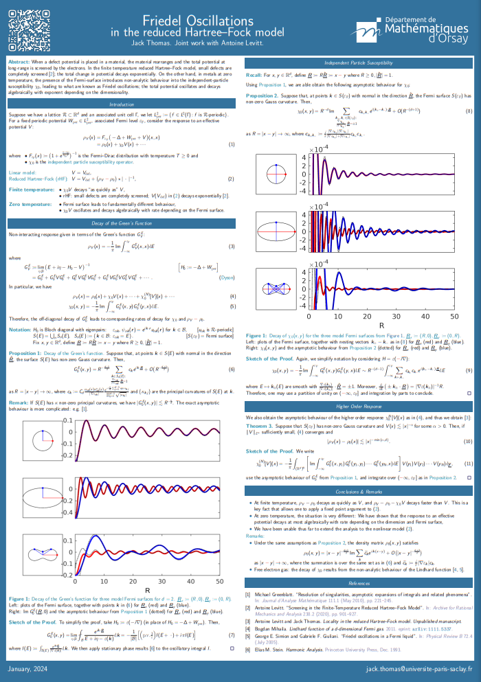
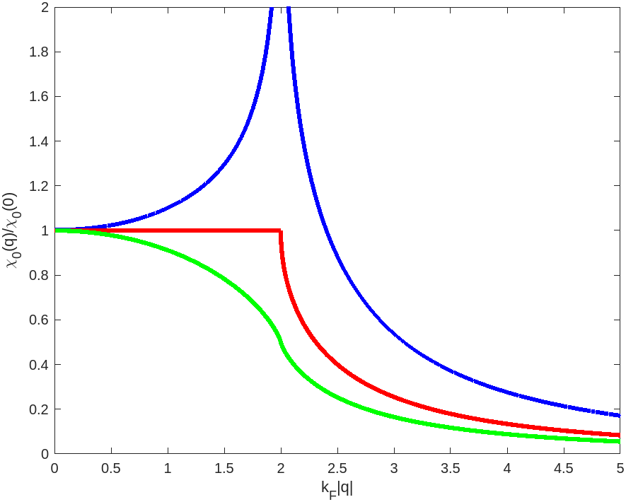Figure 1. Lindhard function. Plot of the Lindhard function $\chi_0(q)$ for $d = 1$ (blue), $2$ (red), and $3$ (green).

Computing the Fourier transform explicitly, one can show that $\chi_0(x)$ oscillates and has $|x|^{-d}$ decay:

\begin{align} \chi_0(x) &= \left\{\begin{matrix} \tfrac{1}{2\pi} \si \, 2k_\mathrm{F} |x| \quad &\text{if } d = 1 \\ % \tfrac{1}{8\pi} k_{\mathrm{F}}^2\big[ J_0 Y_0 + J_1 Y_1\big]( k_\mathrm{F} |x| ) &\text{if } d = 2 \\ % \tfrac{1}{4} \tfrac{1}{(2\pi)^3}\big[ 2 k_\mathrm{F} \cos2 k_\mathrm{F} |x| - \frac{\sin2 k_\mathrm{F} |x|}{|x|} \big] |x|^{-3} % &\text{if } d = 3 \end{matrix} \right\} \\ % &= \tfrac{1}{2} k_\mathrm{F}^{d-2} \frac{\sin (2k_{\mathrm{F}} |x| + (d-2)\tfrac{\pi}{2})}{(2\pi \, |x|)^d} % + O\big( |x|^{-(d + 1)} \big) \tag{4}\label{eq:chi_0(r)} \end{align} as $|x| \to \infty$. Here, $\si(x) \coloneqq - \int_x^\infty \frac{\sin t}{t} \mathrm{d}t$ is the sine integral and $J_n,Y_n$ are Bessel functions of the first and second kind, respectively. Using the asymptotic behaviour of these special functions we obtain (\ref{eq:chi_0(r)}) as $|x|\to\infty$: