16  Galerkin Method and Finite Elements

Lecture 16

Note

I encourage you to play around with the juptyer notebook for this lecture - you can copy the code with the this notebook button on the side of this page.

Warning

These notes are mainly a record of what we discussed and are not a substitute for attending the lectures and reading books! If anything is unclear/wrong, let me know and I will update the notes.

Tip

This chapter is mostly based on

• Burden, Faires, and Burden (2015) Chapter 11,
  
• Driscoll and Braun (2018) Chapter 10,
  
• Today: Driscoll and Braun (2018) Galerkin method

16.1 Recap

We are considering linear boundary value problems of the following form:

\begin{align} \mathcal L[u] &:= -u'' + p u' + q u = f &&\text{on } (a,b) \nonumber\\ &u(a)=0, \qquad u(b) = 0 . \tag{BVP} \end{align}

where p, q may be functions of x. We will see that including non-zero boundary conditions is easy (as in the case of finite differences). By approximating the continuous problem with finite differences, we obtained a discrete problem: find U \in \mathbb R^{n+1} (with index starting at 0) such that

\begin{align} \begin{split} &\mathcal L_h [U] = F \\ &U_0 = U_n = 0 \end{split}\tag{$\text{BVP}_h$} \end{align}

where \mathcal L_h depends on the choice of finite difference scheme. Here is the implementation we saw last time:

"""
    fdm(n, p, q, f; a=0,b=1, A=0,B=0)

Approximate the solution to 
    -u′′ + p u′ + q u = 0 on (a,b)
    u(a) = A, u(b) = B
using central finite differences
"""
function fdm(n, p, q, f; a=0.,b=1., A=0.,B=0.)
    # mesh size
    h = (b-a)/n 
    # interior grid points 
    x = [ a + j *(b-a)/n for j ∈ 1:n-1 ] 

    # Finite Difference Coefficients
    # (using a second order central difference) 
    d = (2/h^2) * ones(n-1) + q.(x)
    d₋  = (-1/h^2)*ones(n-2) - p.(x[2:end])/(2h)
    d₊  = (-1/h^2)*ones(n-2) + p.(x[1:end-1])/(2h)
    Lh = Tridiagonal(d₋, d, d₊)
    F = f.(x)
    F[1] += (1/h^2 + p(x[1])/(2h))*A
    F[end] += (1/h^2 - p(x[end])/(2h))*B
    U = Lh \ F

    # add the boundary conditions
    x = [a, x..., b]
    U = [A, U..., B]

    return x, U
end;

Today, we will look at an alternative approach involving approximating integrals instead of derivatives.

16.2 Galerkin Method

The content of this lecture is mainly contained in Driscoll and Braun (2018) Galerkin method.

We will consider second order linear equations but now written in a slightly different form (that will be more convenient for us):

Exercise 16.1 Show that we can write -u'' + p u' + q u = g as -(\alpha u')' + \beta u = f for some \alpha, \beta, f depending on p,q,g.

Hint: Use the integrating factor e^z where z is a function with z' = -p.

For the rest of this lecture, we will consider: For fixed data \alpha,\beta,f, find u such that

\begin{align} &- (\alpha u')' + \beta u = f \qquad \text{on } (a,b) \nonumber\\ &u(a) = 0, \quad u(b) = 0. \tag{BVP} \end{align}

We assume that \alpha has a continuous derivative, \alpha(x)\geq c>0, \beta is continuous with \beta(x) \geq 0, and f is square integrable \int_a^b |f|^2 < \infty.

16.2.1 Weak formulation

Notice that, if u solves (BVP) and v is a smooth function with v(a) = v(b) = 0, then multiplying (BVP) by v and integrating, we have

\begin{align} (f,v) &:= \int_a^b f v \nonumber\\ &= \int_a^b \left[ - (\alpha u')' + \beta u \right] v \, \mathrm{d}x \nonumber\\ % &= - \alpha(x) u'(x) v(x) \Big|_a^b \nonumber\\ % &\qquad + \int_a^b \left[ \alpha(x) u'(x) v'(x) + \beta(x) u(x)v(x) \right] \mathrm{d}x \nonumber\\ % &= \int_a^b \left[ \alpha(x) u'(x) v'(x) + \beta(x) u(x) v(x) \right] \mathrm{d}x \nonumber\\ % &=: \mathcal A(u,v). \end{align}

Here, we have integrated by parts in the first term.

We will let V be a space of functions v satisfying the boundary conditions v(a) = v(b) = 0 and for which we can define \mathcal A(u,v) for all u,v \in V (it takes a bit more work to define exactly what we mean by V - see a course including Sobolev spaces - it is some space that includes smooth funcions satisfying the boundary conditions).

The weak formulation of the problem can be written as: seek u\in V such that

\begin{align} \mathcal A(u, v) = (f, v) \tag{weak} \end{align}

for all v\in V.

Exercise 16.2 Take u,v, w\in V and \lambda\in\mathbb R. Explain why \mathcal A is

• Positive: \mathcal A(u,u) \geq 0,
  
• Symmetric: \mathcal A(u,v) = \mathcal A(v,u),
  
• Bilinear: \mathcal A(u+ \lambda w,v) = \mathcal A(u,v) + \lambda\mathcal A(w,v) and \mathcal A(u, v+\lambda w) = \mathcal A(u,v) + \lambda\mathcal A(u,w),

16.2.2 Aside: Rayleigh-Ritz Approach

Exercise 16.3 Explain why minimising I(u) := \frac{1}{2} \mathcal A(u,u) - (f,u) over u \in V is equivalent to solving \mathcal A(u,v) = (f,v) for all v\in V.

Hint: If u is a minimiser and v\in V, then

\begin{align} I(u) &\leq I(u + \lambda v) \nonumber\\ % &= \frac12 \mathcal A(u + \lambda v, u + \lambda v) - (f,u + \lambda v) \nonumber\\ % &= I(u) + \lambda[\mathcal A(u,v) - (f,v)] + \frac{\lambda^2}{2} \mathcal A(v,v) \end{align}

Explain why this means that \mathcal A(u,v)=(f,v). [this is the Euler-Lagrange equation (first order condition) for the minimisation problem].

16.2.3 Galerkin approach

The idea behind the Galerkin method is to solve \mathcal A(u,v) = (f,v) over a finite dimensional space of functions V_h := \mathrm{span}\{\phi_1,\dots,\phi_m\}:

\begin{align} V_h = \left\{ v_h = \sum_{j=1}^m c_j \phi_j : c_j \in \mathbb R\right\} \end{align}

(V_h is the space spanned by all linear combinations of the \phi_j). Later, h will denote the spacing of a grid but for now h just means that V_h is any discretisation of the problem.

That is, we are considering the problem: Find u \in V_h such that \mathcal A(u,v) = (f,v) for all v \in V_h.

Exercise 16.4 Explain why this problem is equivalent to: Find u \in V_h such that \mathcal A(u,\phi_i) = (f,\phi_i) for all i=1,\dots,m.

Since, we are considering u \in V_h, we may write

\begin{align} u(x) = \sum_{j=1}^m u_j \phi_j(x). \end{align}

Since \mathcal A is linear in the first component, we want to solve

\begin{align} \mathcal A(u, \phi_i) = \sum_{j=1}^m u_j \mathcal A(\phi_j,\phi_i) % = (f,\phi_i) \end{align}

for all i = 1,\dots,m.

Exercise 16.5 Show that this can be written as the matrix equation

\begin{align} &Au = F \qquad \text{where} \nonumber\\ &A_{ij} := \mathcal A(\phi_i,\phi_j), \quad F_i := (f,\phi_i). \nonumber \end{align}

As a result, we have

\begin{align} A_{ij} &= K_{ij} + M_{ij} \nonumber\\ K_{ij} &= \int_a^b \alpha(x) \phi_i'(x) \phi_j'(x) \, \mathrm{d}x \nonumber\\ % M_{ij} &= \int_{a}^b \beta(x) \phi_i(x) \phi_j(x) \, \mathrm{d}x \end{align}

K is known as the stiffness matrix and M is the mass matrix.

As a result, we have taken the continuous problem (find u\in V such that \mathcal A(u,v) = (f,v) for all v\in V) and approximated it by a discrete problem (find u\in V_h such that \mathcal A(u,v) = (f,v) for all v\in V_h) that can be written as linear system of equations Au = F. Since we are now in “Linear Algebra World”, we can use results from Chapter 2: Iterative Methods (and last semester Chapter 5: Direct Methods) to solve this system of equations.

16.2.4 Finite elements

In order to approximate the solution of -(\alpha u')' + \beta u = f, “all” we have to do is (i) choose a space V_h, (ii) build the matrices K, M and the vector F, and (iii) solve a linear system of equations.

Step 1. The finite element method involves choosing V_h to be a space of peicewise polynomials (splines) defined relative to some mesh. The simplest possible choice are piecewise linear functions defined on the equispaced grid x_j = a + jh := a + j\frac{b-a}{n} for j=0,\dots,n. We define \phi_i to be linear on each I_j := [x_{j-1},x_j] and cardinal: \phi_i(x_i) = 1 and \phi_i(x_j) = 0 for all j\not=i.

Exercise 16.6 Write down the definition of \phi_j(x).

Here’s a plot of a couple of these functions:

a, b, n = 0, 1, 5 
h = (b-a)/n
# mesh: x_1, ..., x_{n-1}
X = [a + j*h for j ∈ 0:n] 

φ(i,x) = max(0, 1-abs( (x-X[i+1])/h ) )

P = plot( x -> φ(1,x), a, b; 
    ylims=[-.15,1], label=L"\phi_1(x)", lw=2)
plot!( x -> φ(2,x), a, b; label=L"\phi_2(x)", lw=2)
scatter!( X, zeros(n+1), label="grid", color=:black)
for i = 0:n
    annotate!( X[i+1], -.05, text(L"x_%$i") )
end

P

Remark 16.1. The two dimensional analog of these hat functions look like this:

Courtesy of Núñez Ramos (2025.)

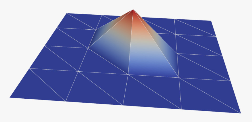
One often uses triangles (as in this case) but you can also use rectangles, hexagons, …

One can write any piecewise linear function on the mesh with zero boundary conditions as a linear combination of \phi_j for j=1,\dots,n-1. Moreover, the piecewise linear interpolation of some function f on the grid can be written

\begin{align} If(x) &= \sum_{j=0}^n f(x_j) \phi_j(x) \end{align}

We show this in the following plot:

f(x) = x^2 * sin(2π * x)
If(x) = sum( f(X[i+1]) * φ(i,x) for i ∈ 0:n )

plot(f, 0,1, label=L"f")
plot!(If, label=L"If")
scatter!( X, f.(X), label=L"( x_j, f(x_j) )", color=:black )

The “finite elements” in this case refer to the intervals I_j = [x_j,x_{j-1}]. In 2d, one often uses triangles, ….

Step 2. Recall that we want to build the matrices K, M and the vector F:

\begin{align} K_{ij} &= \int_a^b \alpha(x) \phi_i'(x) \phi_j'(x) \mathrm{d}x \nonumber\\ M_{ij} &= \int_a^b \beta(x) \phi_i(x) \phi_j(x) \mathrm{d}x \nonumber\\ F_i &= \int_a^b f(x) \phi_i(x) \mathrm{d}x \end{align}

(and then solve (K+M)u = F to obtain a (piecewise linear) approximation to the exact solution to the continuous problem).

Unless \alpha, \beta, f are “simple”, in practice one implements various quadrature schemes (Chapter 4 of Math 5485) to approximate these integrals. Perhaps the easiest thing you can do is, on each interval I_k = [x_{k-1}, x_k], replace the function \alpha, \beta, f with a constant and evaluate the resulting integral exactly:

\begin{align} K_{ij} &\approx \sum_{k=1}^n \frac{\alpha(x_{k-1})+\alpha(x_k)}{2} \int_{I_k} \phi_i'(x) \phi_j'(x) \mathrm{d}x \nonumber\\ % M_{ij} &\approx \sum_{k=1}^n \frac{\beta(x_{k-1})+\beta(x_k)}{2} \int_{I_k} \phi_i(x) \phi_j(x) \mathrm{d}x \nonumber\\ % F_i &\approx \sum_{k=1}^n \frac{f(x_{k-1})+f(x_k)}{2} \int_{I_k} \phi_i(x) \mathrm{d}x \end{align}

Exercise 16.7 Show that

\begin{align} \int_{I_k} \phi_i'(x) \phi_j'(x) \mathrm{d}x % &= \frac1h \begin{cases} 1 & \text{if } i = j \in \{k, k-1\} \\ -1 & \text{if } \{i,j\} = \{k,k-1\}\\ 0 & \text{otherwise} \end{cases} \end{align}

In particular, if \alpha(x) = \rm const., then

\begin{align} K_{ij} &= \frac1h \begin{cases} 2 & \text{if } i = j \nonumber\\ -1 & \text{if } |i-j| \nonumber\\ 0 & \text{otherwise}. \end{cases} \end{align}

What do you notice about this matrix?

Exercise 16.8 Show that

\begin{align} \int_{I_k} \phi_i(x) \phi_j(x) \mathrm{d}x % &= \frac{h}{3} \begin{cases} 1 & \text{if } i=j \in \{k,k-1\}\\ \frac12 & \text{if } \{i,j\} = \{k,k-1\}\\ 0 &\text{otherwise}. \end{cases} \end{align}

Show that

\begin{align} \int_{I_k} \phi_i(x) \mathrm{d}x = \frac{h}{2}\begin{cases} 1 &\text{if } i \in \{k,k-1\} \\ 0 &\text{otherwise} \end{cases} \end{align}

Step 3. Solve the linear system of equations (we use the built in function u = A \ F) - see Chapter 2!

We implement this here:

"""
    fem(n, α, β, f; a=0, b=1)

Approximate the solution to 
    -(α u′)′ + β u = f on (a,b)
    u(a) = 0, u(b) = 0
using finite element method with hat functions
"""
function fem(n, α, β, f; a=0, b=1)
    h = (b-a) / n
    x = a .+ h .* (0:n)

    α_av = (α.(x[1:n])+α.(x[2:n+1]))/2
    β_av = (β.(x[1:n])+β.(x[2:n+1]))/2
    f_av = (f.(x[1:n])+f.(x[2:n+1]))/2

    K_d  = [ (α_av[i]+α_av[i+1])/h for i ∈ 1:n-1 ]  
    K_dl = [ -α_av[i+1]/h for i ∈ 1:n-2 ]    
    K = SymTridiagonal(K_d, K_dl)

    M_d = [ h/3 *(β_av[i] + β_av[i+1]) for i ∈ 1:n-1 ]
    M_dl = [ h/6 *β_av[i+1] for i ∈ 1:n-2 ]
    M = SymTridiagonal(M_d, M_dl)
    
    F = [ (h/2) * ( f_av[i] + f_av[i+1] ) for i = 1:n-1 ]
   
    u = (K+M) \ F
    u = [0; u; 0]    
    return x, u
end

fem

Example 16.1 (Driscoll and Braun (2018) Example 10.6.2) Let’s apply this to the following problem

\begin{align} &-(x^2 u')' + 4u = \sin \pi x && \text{on }(0,1) \nonumber\\ % &u(0) = u(1) = 0 \end{align}

• Write this in the form -u'' + p u' + q = f,
• Let’s see how our finite element method compares to the finite difference method we had last time:

p(x) = -2/x
q(x) = 4/x^2
g(x) = sin(π*x)/x^2    

α(x) = x^2
β(x) = 4
f(x) = sin(π*x)

x, u = fem(25, α, β, f)
plot(x, u; 
     label="finite element method", markersize=2, m=2)

x2, u2 = fdm(25, p, q, g)
P1 = scatter!(x2, u2;  
     label="finite difference method", markersize=2)

Here is the error curve for both:

# we measure the error on the grid egrid:
egrid = range(0,1,500)

# compute a reference solution to compute the error against
x, u = fem(2^15, α, β, f)
u_e = linear_interpolation(x, u)

nn = [2^j for j∈2:12]
err_fem = zeros(length(nn))
err_fdm = zeros(length(nn))

for (i,n) ∈ enumerate(nn)
    x, u = fem(n, α, β, f)
    uf = linear_interpolation(x, u)
    err_fem[i] = abs.( maximum(uf.(egrid) - u_e.(egrid)) ) 

    x, u = fdm(n, p, q, g)
    uf = linear_interpolation(x, u)
    err_fdm[i] = abs.( maximum(uf.(egrid) - u_e.(egrid)) ) 
end

plot( nn, err_fem;
    xaxis=:log,yaxis=:log, m=2, xlabel=L"n", ylabel="error",
    label="FEM" )
plot!( nn, err_fdm;
    label="FDM", m=2 )
plot!( nn[3:end], nn[3:end].^(-2), linestyle=:dash, label=L"O(h^2)")

Exercise 16.9 Now suppose we want to solve the BVP with non-zero boundary conditions:

\begin{align} &-(\alpha u')' + \beta u = f \qquad \text{on } (a,b) \nonumber\\ &u(a) = A, \qquad u(b) = B. \end{align}

Show that

\begin{align} u(x) &= v(x) + \theta x + \varphi \end{align}

with \theta := \frac{B-A}{b-a} and \varphi := \frac{Ab - Ba}{b-a} and v solves the problem

\begin{align} &-(\alpha v')' + \beta v = f + \theta \alpha' - \beta( \theta x + \varphi ) \qquad \text{on } (a,b) \nonumber\\ &v(a) = 0, \qquad v(b) = 0. \end{align}

How can you use this and the function fem() to approximate the solution to the BVP with non-zero boundary conditions?

a, b, A, B = 0, 1, 0, 1/2 
α(x) = x^2
α′(x) = 2x
β(x) = 4
f(x) = sin(π*x)

θ = (B-A)/(b-a)
ϕ = (A*b - B*a)/(b-a)

# transformed RHS 
f_shift(x) = f(x) + θ*α′(x) - β(x)*(θ*x + ϕ)

x, v = fem(5, α, β, f_shift; a, b)
u = v + θ*x .+ ϕ
P = plot(x, u; 
     label="finite element method", markersize=2, m=2)

x2, u2 = fdm(5, p, q, g; a, b, A, B )
plot!(x2, u2; 
     label="finite difference method", markersize=2, m=2)

TipTO-DO

• Today: Driscoll and Braun (2018) Galerkin method
• Take a look at the suggestions for Presentations/Posters/Papers and sign up to present,
• Read through the proofs/exercises from this lecture and Monday,
  
• (Sign-up to office hours if you would like)

Previous reading:

• Chapter 1 reading:
  • Burden, Faires, and Burden (2015) sections 5.1 - 5.6,
    
  • Driscoll and Braun (2018) zero stability
• Chapter 2 reading:
  • Recap matrices: sections 7.1 - 7.2 of Burden, Faires, and Burden (2015)
  • Jacobi & Gauss-Seidel: section 7.3 Burden, Faires, and Burden (2015)
    
  • CG: section 7.6 Burden, Faires, and Burden (2015)
• Chapter 3 reading:
  • Sections 11.1 - 11.2 of Burden, Faires, and Burden (2015): shooting methods

Burden, Richard L., Douglas J. Faires, and Annette M. Burden. 2015. Numerical Analysis. 10th ed. CENGAGE Learning.

Driscoll, Tobin A, and Richard J Braun. 2018. Fundamentals of Numerical Computation. https://fncbook.com/.

Núñez Ramos, Cristhian. 2025. “Symplectic Hamiltonian Hybridizable Discontinuous Galerkin Methods for Shallow-Water Equations.” PhD thesis, Pontificia Universidad Catolica de Chile. https://doi.org/10.7764/tesisuc/mat/105265.